Table of Contents
4-1 Surface Water and Groundwater
Read Chapter 13 in Physical Geology.
Clean fresh water is our most precious resource. We cannot survive without it, and therefore, we should all know where our water comes from and what could put it at risk. In this first section of Unit 4, we will be looking at the water cycle, surface water, flooding, and groundwater.
Chapter 13 in the textbook is about streams and floods. We will be covering only part of that material in this section, including the hydrological cycle, flow of water on the surface, and the causes and effects of floods.
The hydrological cycle—illustrated in Figure 13.1.1 and described in Section 13.1—is familiar to most people. Water is stored in various reservoirs—the atmosphere and oceans, lakes and streams, soil and vegetation, glacial ice and groundwater—and is transferred from one to another with the help of energy from the Sun (evaporation) and gravity (mostly stream and groundwater flow). Figure 13.1.2 provides a way of visualizing the amounts stored in these various reservoirs. The key point is that 97% of our water is salty water in the ocean, a further 2% is held in glacial ice, and fresh water that we can use makes up the remaining 1%. Over 90% of that is stored as groundwater.
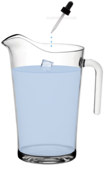
You might find it instructive to do the experiment represented by Figure 13.1.2 in the textbook.
Pour 970 mL of water into a jug, and then add 34 g (7 teaspoons) of salt and stir. That’s how salty ocean water is. Taste it! A teaspoon of it won’t hurt you. Now add a single ice cube to represent all of the frozen water on Earth, and two more teaspoons of water to represent all of the water stored underground.
Now we need to add three more drops to represent the fresh water in all of the Earth’s lakes, streams, and wetlands plus all of the water in the atmosphere, including clouds. If you don’t have an eye-dropper, you could turn your tap down to the point where it’s just dripping, and capture three drops in a spoon.
© Steven Earle. Used with permission.
Water moves between these reservoirs, and you can get a feel for the rate of transfer from one reservoir to another by completing Exercise 13.1.
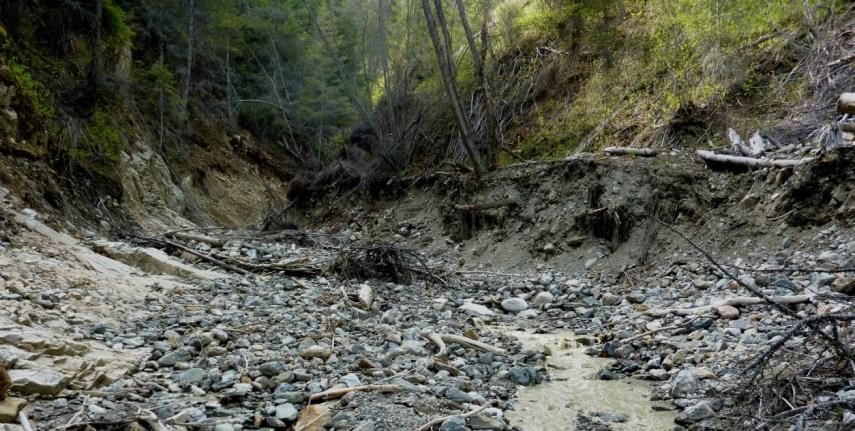
Section 13.2 examines the topic of streams and drainage basins. A stream flows within a channel that is typically created by the stream itself through erosion of rock (Figure 4-1). A network of small streams that converge to make a large stream defines a drainage basin, which is an area of land within which all of the surface water eventually flows into the main stream. Drainage basins are illustrated in Figures 13.2.1 and 13.2.3.
As discussed in Section 13.5, all streams show significant variations in discharge (volume of water passing a point per unit of time). In cold parts of Canada, the greatest flows are experienced in spring or early summer when melting is at its peak. This flow is illustrated in Figure 13.5.1 for the Stikine River in northwestern BC, which has a discharge of under 100 m3/s in the cold of winter, and peaks at over 2000 m3/s in May and June. In the southern coastal regions of BC, peak discharges are typically in mid-winter due to heavy winter rains (Figure 13.5.2).
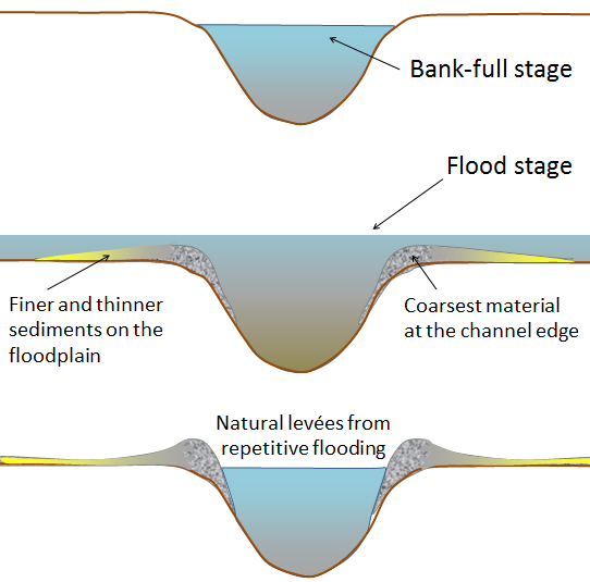
As a result of extreme rainfall events, or of rain storms that coincide with strong melting, discharge levels can be so great that streams fill their channels to the brim, and then spill over into the surrounding flood plain. This phenomenon is illustrated in Figure 4-2. The flow velocity reaches a maximum as a stream approaches its “bank full” stage, and then as soon as it pours over into the flood plain, the velocity drops significantly (because more area is available to accommodate the flow volume). When this happens, sediments are deposited on the banks and further out into the flood plain. The natural levees that form in these situations can help to limit future flooding. On many rivers, such as the lower part of the Fraser River, natural levees have been supplemented or replaced by man-made dykes.
Constructing dykes on rivers is controversial for many reasons. First, it’s expensive; second, dyking in one area can lead to worse flooding in other areas; and third, flooding is what makes river-valley land fertile in the first place, so putting an end to floods is not in the best interests of farmers or the people that eat the food they produce.
In Section 13.5, read about the 2013 floods in southern Alberta, which, like many flood events in Canada, were caused by a combination of snow-melt and heavy rain.
Completing Exercise 13.5 will help you to understand the significance of this and other floods on the Bow River.
Answer the review questions 1, 2, 11, 12, and 13 at the end of Chapter 13, and check your answers in Appendix 2 in the textbook.
Read Chapter 14 in Physical Geology.
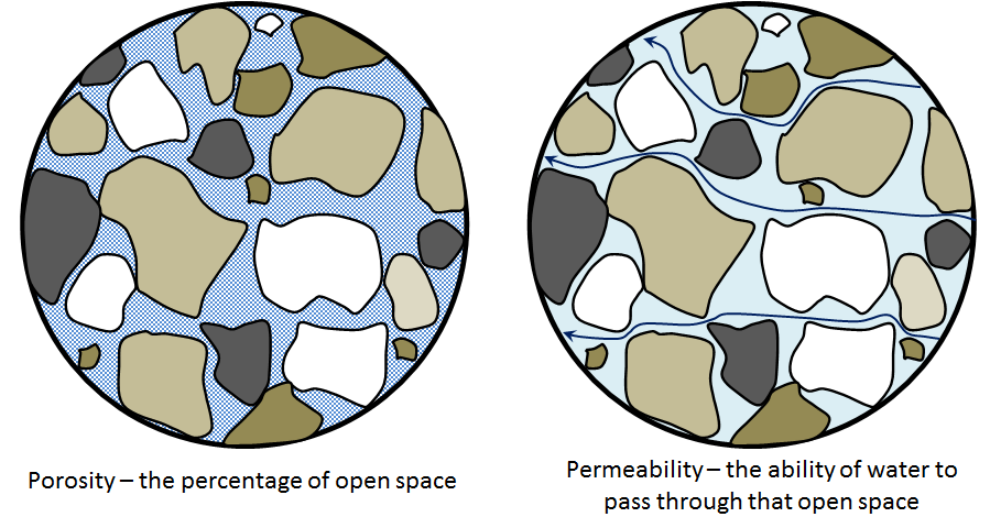
Groundwater is examined in Chapter 14, which begins with a discussion of porosity and permeability (Figure 4-3). As shown in Figure 14.1.1, most unconsolidated materials have porosities in the 30 to 60% range, whereas most solid rocks have porosities of less than 30%—in many cases much less. Porosity is an important indicator of how much water can be held in rock or unconsolidated material, but the more significant factor that controls groundwater accessibility is the permeability of these materials, in other words, how easily water can flow through them.
As shown on Figure 14.1.2, geological materials have a very wide range of permeability values from 0.000000000001 m/s to 1 m/s (i.e., K = 10-12 to K = 100 m/s). Permeability is denoted by the letter “K.” Unconsolidated materials are generally more permeable than solid rocks, and the coarser they are, the more permeable. Unfractured igneous and metamorphic rock and mudstone have the lowest permeabilities, and well-fractured rocks tend to be much more permeable than unfractured rocks.
A strong correlation doesn’t necessarily exist between porosity and permeability. For example, while clay is one of the most porous of materials, it also is one of the least permeable. As described in the textbook, clay particles are very small and closely packed together. Its porosity is made up of many tiny spaces between the grains, and while those spaces can hold lots of water, almost all of it is tightly held by the mineral surfaces and cannot easily move within the clay deposit.
A body of rock or unconsolidated material that has good permeability is known as an aquifer, which is what people look for when they want to extract groundwater. The best way to find a good aquifer is to understand the geology of an area, and specifically the nature of the rocks and unconsolidated materials that might be underneath you. Of course, this is not a guarantee that you’ll find what you’re seeking, since the permeability of a specific rock unit can vary from place to place. In some cases, permeability is related to fractures or bedding planes whose locations are very difficult to predict.
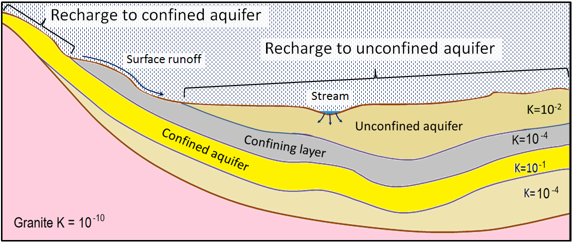
As illustrated in Figure 4-4 (which is similar to Figure 14.1.4 in the textbook), aquifers are described as unconfined if they are open to the surface, or confined if they are covered by a layer of impermeable material. In Figure 4-4, rain is depicted by vertical dashes, and a proportion of it will infiltrate into the ground and recharge the aquifer. Since an unconfined aquifer is exposed at the surface everywhere, it has more opportunity to be recharged by rain than a confined aquifer. An unconfined aquifer also can be recharged directly by a body of surface water (such as a stream) or by surface runoff.
The concept of a water table is introduced in Section 14.2, which describes it as the upper surface of a zone where all of the porosity is filled (i.e., saturated) with water. Be careful not to think of the water table as an object—you can’t pump water from a water table! However, you can pump water from a body of saturated rock, and the water table is just the upper surface of the part of that rock that is saturated. As shown in Figure 14.2.1, a water table isn’t typically horizontal. In this example, the water table is a few metres below the ground surface near to the top of the hill, but is at surface adjacent to a stream. The water table slopes towards the stream, and an 8 m difference exists in the elevation between the well and the stream. That difference in elevation, divided by the horizontal difference between the two points (100 m), is called the hydraulic gradient, which is denoted by the letter “i” (in this case, i = 8/100 = 0.08). The hydraulic gradient also can be described as the slope of the water table between those two points.
Section 14.2 also makes the point that if we know the hydraulic gradient and the permeability of an aquifer, we can estimate the rate of groundwater flow within an aquifer by using Darcy’s equation: V = K * i.
You can practise estimating groundwater flow rates and travel times by completing Exercise 14.1. Bear in mind that in this example and the one described in the textbook, the hydraulic gradients and permeabilities are on the high end of the spectrum found in nature. In other words, these flow rates—in the order of cm/day to m/day—are many times higher than would be typical in most natural settings.
Groundwater flow paths and rates are predictable, but not simple. Figure 14.2.5 shows that groundwater doesn’t flow in a straight line from an area where the hydraulic gradient is high to where it is low. Furthermore, in many situations, it can seem to flow “uphill.”
Extraction of groundwater is typically done using wells that are constructed in unconsolidated material or rock using a drilling machine like the one in Figure 14.3.1. Once the well has been completed, water can flow into it through the surrounding material, and a pump can be used to extract the water. As water is pumped out, it is typical for a cone of depression to form around the well (Figure 14.3.2), and if the pumping continues at a rate faster than the water can flow in, the well may go dry. In this case, when the pumping stops, the water level should recover.
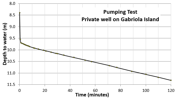
An example of a water-level drawdown in a well during pumping is shown in Figure 4-5. When this low-capacity well was pumped at a relatively slow rate (3 litres per minute), the water level dropped from 8.4 m to 9.7 m in only 2 minutes, which produced a cone of depression of about 2.3 m that allowed the water to flow more quickly into the well. Nevertheless, the rate of inflow was not sufficient to keep up with the rate of pumping, and the water level continued to drop at a consistent rate for the next 2 hours.
Wells are very useful for monitoring groundwater levels, and a large network of monitoring wells exists across British Columbia and elsewhere in Canada because it’s important for us to know the status of our groundwater resources. The well record shown in Figure 14.3.7 is typical for many wells in coastal British Columbia, with relatively high levels in the spring, peaking in April or May, dropping through the dry period of the summer and into the fall, and then starting to rise again in October or November. In colder regions, the peak comes later in the spring.
You can learn about the groundwater in your region by completing Exercise 14.3. If you don’t live in British Columbia, you may be able to find comparable data for your region.
It is noted in Section 14.4 that groundwater has the distinct advantage of not being as easily contaminated as surface water (especially by bacterial contaminants), but also the moderate disadvantage of having higher concentrations of many dissolved elements compared with surface water. In some cases, these elements can be present at dangerous levels, and in others just to the extent that the water doesn’t taste as good as we would like it to. Some examples are provided in the textbook.
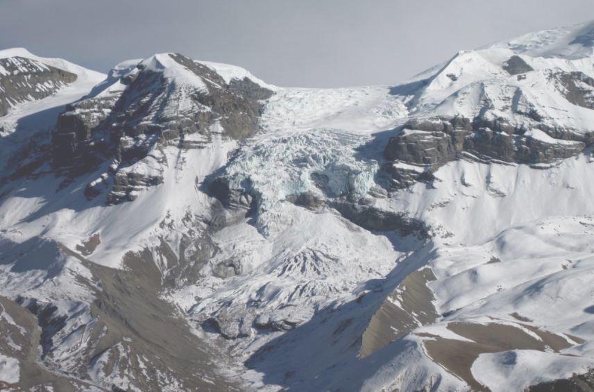
It is critical for us to protect our groundwater resources because they are generally more reliable than surface water resources, and, as the climate continues to change, we may find that we cannot rely on our surface water supplies. One example of this shift is the rapid disappearance of glaciers everywhere in the world. In many locations, surface water supplies are significantly supplemented by the melting of glacial ice during the dry summer. Once those glaciers are gone, that component of the water supply will be gone too. Even where glacial melting is not part of the supply, snow melting typically is, especially in Western Canada. In recent years, snow packs have been at their lowest levels on record.
Please answer the review questions at the end of Chapter 14.